Files
der-1.gif
der-2.gif
dt-1.gif
dt-2.gif
dt-20.gif
dt-3.gif
dt-4.gif
fig-1.gif
index.html
lim-1.gif
MatlabPlotting.mp4
MatlabPlottingR2018a.mp4
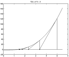
newtons-method.gif
next_motif.gif
plt-8.gif
plts-1.gif
plts-2.gif
plts-3.gif
plts-4.gif
plts-5.gif
plts-6.gif
plts-7.gif
plts-7a.gif
previous_motif.gif
projectile-motion.mp4
projectile-motionR2018a.mp4
salary.mp4
salaryR2019a.mp4
shrt-1.gif
sin365.mp4
sin365R2018a.mp4
test.gif
tutorial-pieces.html
tutorial.html
tutorial001.gif
tutorial001.html
tutorial002.gif
tutorial002.html
tutorial003.gif
tutorial003.html
tutorial004.gif
tutorial004.html
tutorial005.gif
tutorial005.html
tutorial006.gif
tutorial006.html
tutorial007.gif
tutorial007.html
tutorial008.gif
tutorial008.html
tutorial009.gif
tutorial009.html
tutorial010.gif
tutorial010.html
tutorial011.gif
tutorial011.html
tutorial012.gif
tutorial012.html
tutorial013.gif
tutorial013.html
tutorial014.gif
tutorial014.html
tutorial015.gif
tutorial015.html
tutorial016.gif
tutorial017.gif
tutorial018.gif
tutorial019.gif
tutorial020.gif
tutorial021.gif
tutorial022.gif
zer-1.gif
zer-1a.gif
zer-2.gif
zer-3.gif


3 How to work with numbers in MATLAB
To study Calculus using MATLAB we use a few features of MATLAB that allow us to store numbers, and lists of numbers.For a quick introduction click below, for a more thorough one, read on.
3.1 Quick introduction
A quick introduction to data typesWe make use of two types of data in using MATLAB for calculus: numbers, or scalars and lists or vectors. The words scalars and vectors are names given in a Linear Algebra course. How do we use these? Let's illustrate with an example:
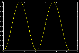
Example: sin2 x plot
Plot the function f(x) = sin2(p x) over the interval [0,2 p]. Answer:
What do we need to do to plot this?
If x was a number say 5, then we would compute f(5) in MATLAB in a manner similar to a what is done on a calculator:
>> sin( pi * 5 ) ^2
ans = 0
However, we will use the plot command. Plotting is discussed in the section of plotting functions . To use the plot command, we need to generate a table of numbers for the x- and y- coordinates. Of course we would like to do this in the easiest way possible.
-
First generate a list of numbers for the x coordinates. One
way to do
this is with the
linspace
command.
>> x=linspace(0,2 * pi); % generates 100 numbers between 0 and 6.28...
To take a peak at what you have done type (its a mess)>> x % yikes 100 numbers!
- Next we generate the y values corresponding to the x
coordinates. So for each value in the list for x we need to
create the value of f(x). That is we multiply by p, then we
find the sine, then we square. Now we want to do this for all the
values in the list at once and here is where we need to be
careful. If x was just a number or
scalar
, say x=5, we
would simply type what we have above.
>> sin(pi*x)^2 % Won't work for out x!!
However, this won't work as x is a list of numbers. And we need to tell MATLAB to treat it the right way. So we do this in steps:-
multiply x by p. This is a number times a list. MATLAB does
this as you would expect
>> pi * x % multiplies each element of x by pi
- find the sine of the new number. The new number is a list,
so we need to take the sine of a list of numbers. Again MATLAB is
smart enough to know how to do this:
>> sin(pi*x) % finds the sine of each element
- Finally we need to take the square. We can think of this as
multiplying two lists of numbers. How do we want this to be
done? Now it gets interesting. In linear algebra there is a very
common way to multiply vectors (or lists) called the
dot-product
. Here is
an example:
(1,2,3) � (1,3,5) = 1 � 1 + 2 � 3 + 3 � 5 = 22Notice, you match up the corresponding terms, multiply these and then add. This is the default way that MATLAB multiplies matrices .
We want something different: We want to match up corresponding terms, multiply and get a list when all is said and done. To do this in MATLAB you tell the multiplication to work ``element by element''. The special command for this is a ``.'': a period or a ``dot''. Here's how it works with the simple example above:>> [1,2,3] * [1,3,5] % gives an error >> [1,2,3] * [1,3,5]' % returns 22. the ' is transpose % (this is the dot product) >> [1,2,3] .* [1,3,5] % what we want a list ans = 1 6 15which is the list [1,6,15]. To multiply we put a ``.'' in front. As well this is necessary for division ./ and exponentiation (.^). Thus our plotting commands could be:>> x = linspace(0,2*pi); >> y = (sin(pi*x)).^2; % using the .^ notation as the % sin(pi*x) is a list >> plot(x,y); % enough already, make the plot
-
multiply x by p. This is a number times a list. MATLAB does
this as you would expect
3.2 Numbers and lists in MATLAB
The language of MATLAB is taken from that of Linear Algebra. It is important to understand a few different types of data. First we are all familiar with numbers. You should know the difference between the integers, the rational numbers, the real numbers and you may know the complex numbers. In linear algebra of MATLAB we call these scalars .Why do we need to give these a separate name? We also want to talk about lists or arrays of numbers. In Linear Algebra we may call these lists vectors . There is a mathematical connection made between a vector, which is a way to represent a magnitude and a direction, and a point on the graph. This is why MATLAB uses coordinates to represent vectors. An example might be the coordinates of a point on the graph: (4,5), or in 3 dimensions (3,4,5). Or, a list of x-coordinates that we wish to find the y coordinates for. As well, we can use a list as a shortcut to represent polynomials: for example f(x)= 5x2 - 6x + 12 could be associated with the list (5,-6,12).
This is really confusing if you are not careful. Let's look at a table of some different ways a mathematician like yourself can think of the list of numbers (1,2):
| (1,2) | the point (1,2) in the Cartesian plane |
| (1,2) | the vector associated with the directed line segment (0,0),(1,2) |
| � 1,2� | the same vector, only in another notation |
| [1,2] | the MATLAB notation for a row vector |
| [1;2] | the MATLAB notation for a column vector |
| [1,2] | a coding for the polynomial 1x + 2 |
| [1,2] | a way to represent the equation 1x = 2 in linear algebra |
We can also speak of two-dimensional arrays of data, much like the way we reference elements of a spread sheet. We may need two indices to speak about something: such as the first column and 2nd row has a value of 10. In shorthand we might write something like a21=10 and understand this to be shorthand for what we have in mind. Such things are referred to as matrices . Another example might be if we have two lists, say 10 x-coordinates and 10 y-coordinates. Then we might want the 8th x coordinate or the 6th y-coordinate. These could easily be referred to by a81 or a62. a final example is to represent a system of equations.
Example: The system of equations
| 7x + 5y + 0.1 z | = 100 |
| x + y + z | = 100 |
|
Now for the fun stuff. We may want to multiply these things together. You should be familiar with addition, subtraction, multiplication and division of numbers or scalars, but you might be surprised to know there are ways of doing such combinations to vectors and matrices as well that are important in many areas of mathematics.
You may ask ``How do we tell MATLAB that we are multiplying a scalar times a vector, or how do we tell MATLAB that we are multiplying a vector times a vector''. MATLAB is as smart as it can be about guessing, but you will have to supply the answer in some cases.
In particular, if in doubt MATLAB will assume you are referring to a matrix. So to really understand how MATLAB works, you need to know what matrix operations are.
3.3 Numbers or scalars
First we need to understand operations between scalars. This is easy as it is simply the arithmetic we are all familiar with.3.3.1 Usual Arithmetic
The simplest MATLAB commands are arithmetic operations which are the familiar operations of your calculator. These are represented by the following symbols: addition (+), subtraction (-),
multiplication (*), division (/), and exponentiation
(^). Try the following commands and observe the MATLAB
responses. After typing each line below remember to hit the
enter key to put MATLAB to work.
>> 3+4                 % ans = 7
>> 5*9                 % ans = 45
>> 8/9                 % ans = 0.8889
>> 5^3                 % ans = 125
>> sin(pi)             % ans = 0. pi is the constant 3.14...
Even better than a calculator, just like in Calculus, we can can make assignment statements to simplify or organize our work. here are some examples:
Example: Assignment to variables
>> a = 7;                       % the variable a is now 7
>> b = 2; a = 5;                % b is 2, and now a is 5
>> c = a - 2;                   % c is now 5-2 or 3
>> a = a + 1                    % a common computer statement.
                                % a is now 5 + 1 or 6
>> a,b,c                        % easy as a,b,c -- prints them out.
>> e = exp(0)                   % e is now e^1=2.71.... (no built-in
                                % constant like pi)
>> log(e)                       % ans = 0
>> x = 2;h=.01                  % define some variables
>> fx = x^2; fxh = (x+h)^2      % f(x) = x^2, fx=f(x), fxh=f(x+h)
>> slope = ( fxh - fx )/h       % slope of secant line
>> r = 5;                       % define the radius
>> area = pi * r^2;             % area of a circle
>> r = 2.5;                     % oops before we had the diameter
>> area = pi * r^2;             % We don't need to retype
                                % use th up-arrow
>> clear(a)                     % clears out the a variable
>> clear                        % clears out all variables
A few comments:
- Since spaces are ignored its a good idea to make your lines easy to
read
>> difficult=exp(sin(x^2-5*x+6*(4-3)))
>> easy = exp( sin( x^2 - 5*x + 6*(4 - 3))) % trust us!
- If a command is followed by a semicolon (;) then MATLAB carries
out the operation but the result will not appear on the screen.
- Once a value is assigned to a variable, MATLAB remembers it until that variable is reassigned or cleared.
3.3.2 Order of Operations
First a ``quick and dirty'' answer, then a more thorough one.When you have a sequence of operations, it is always possible to force them to be performed in a certain order by using parentheses. For example, (5-2)/6 = 3/6=2, or 5-(2/6) = 5 - (1/3) = 14/3. However, one often wants to omit parentheses to avoid typing. MATLAB uses the standard order of priority (precedence) for operations: addition and subtraction have the same priority, as do multiplication and division. Exponentiation has higher priority.
Example: First assign values to a, b, and c as described above. For example:
>> a=8; b=2; c=16;Then we verify
Command                    Numerical Answer       in Math language

>> a - b * c                    -24                 a - (b * c )
>> (a - b) * c                   96                 (a-b)*c
>> a / b / c                    .25                 (a/b)/c
>> a / (b / c)                  64                  a/(b/c)
>> a ^ b * c                    1024                (a^b)*c
>> a ^ (b * c)                  7.9228e+28          a^(b*c)
>> a ^ b ^ c                    Inf                 a^(b^c)
To see a more detailed explanation read on.
MATLAB uses the following symbols for arithmetic operations:
| Operation | Symbol | Precedence | Comment |
| Exponentiation | ^ | 3 | Highest precedence |
| Multiplication | * | 2 | |
| Division | / | 2 | |
| Addition | + | 1 | |
| Subtraction | - | 1 | Lowest precedence |
If an arithmetic expression contains nested parentheses, then the expressions contained within the innermost parentheses are evaluated first. In the absence of parentheses, the precedence rules decide the order of evaluation. The following rules apply:
1. All operations with a higher precedence are carried out before those of lower precedences. Thus exponentiation is carried out first, then comes multiplication and division, and finally, addition and subtraction.
2. If two operations have the same precedence then the operation on the left is carried out first. This is called the left-to-right scan rule.
The examples in the following table show how the precedence rules help interpret arithmetic expressions based on these rules. Try them out on the computer and make sure that you understand how each expression is interpreted.
| Expression | MATLAB value | Interpreted as |
2*3+4*5 |
26 | (2*3)+(4*5) |
2+3*4 |
14 | 2+(3*4) |
(2+3)*4 |
20 | parentheses decides the order |
2/5*4 |
1.6 | (2/5)*4 |
2/(5*4) |
0.1 | parentheses decides the order |
2\^{}3\^{}2 |
64 | (2^3)^2 |
2\^{}(3\^{}2) |
512 | parentheses decides the order |
5/2/4 |
0.625 | (5/2)/4 |
5/(2/4) |
10 | parentheses decides the order |
3.4 Lists or vectors
What is a list or vector ? In MATLAB and linear algebra they are a way to keep track of several values at once. Here is how we can generate them:Example: How to generate lists
  w = [1,3,5,7];                % the list 1,3,5,7
  x = [1;3;5;7];                % take a peek at x and w to see the
                                % difference. A column vector!
  y = 1:2:7;                    % again the list 1,3,5,7
  z = linspace(1,7,4);          % one more time
To generate w and x we used the MATLAB command to
specify a list member by member. The commas create a row
vector
, the semi-colons create a column
vector
. Take
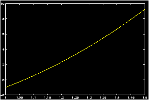
a peek at the values of w and x to see the difference.To generate y we use the colon-operator , a shorthand way to generate evenly spaced values. The format is a:h:b. Which generates evenly spaced numbers starting from a to b in steps of size h. Finally, z is generated using the linspace command which by default generates 100 evenly spaced values between the two points given, in this case 1 and 7. By using a third argument, we specified the number of points, in this case 4.
For more details go click below:
3.4.1 Generating lists of data
We will see how generate lists of data. To be specific, we will call a list of data a vector .- Entering specific numbers
Example: Suppose you have a list of jogging times as follows: 30.45, 29.54, 31.16, 42.33 in minutes and seconds. To store these in a list we could type the following:>> times = [30.45, 29.54, 31.16, 42.33] % notice the [] and the commas , times = 30.450 29.540 31.160 42.330 % a row of numbers
or>> runs = [30.45; 29.54; 31.16; 42.33] % notice the semicolon ; runs = % a column of numbers 30.450 29.540 31.160 42.330There is a distinction made in MATLAB between rows of numbers and columns of numbers (row vectors and column vectors). MATLAB can switch between them with the transpose operator ' for example>> runs' % notice the ' sign runs = 30.450 29.540 31.160 42.330 % a row of numbers
The transpose operator can be useful when displaying your data.
- Extracting data
Suppose I have times entered in above, and I want to know the 1st jogging time. I can get at this as follows:>> times(1) % returns 30.450 >> times(3) % returns 31.160 >> times([1,3]) % returns 30.450 and 31.160
The last line uses a slice of the vector. It finds the 1st and 3rd times. This can be useful.
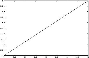
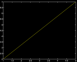
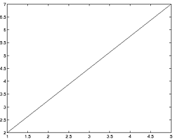
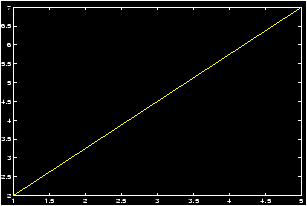
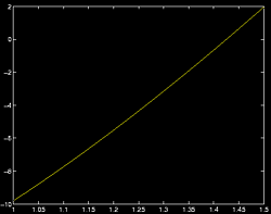
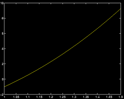
Example: Suppose we want to plot the line connecting (1,2) to (5,7). To plot the line we may want to enter the data as a table:>> x=[1,5];y=[2,7]; % the x-values and y-values
The command>> plot(x,y)
would plot a straight line segment between the points (1,2) and (5,7). What is its slopem = ( y(2) - y(1) )/ ( x(2) - x(1) ) % m = (7 - 2)/(5 - 1) = 1.2500
- evenly spaced numbers
If you had to enter the number 1 through 5 into a list you could
type
x = [1,2,3,4,5]
which isn't too bad, but suppose you had to do 1 through 100. You'd want a shortcut. Fortunately there is one using the colon-operator :x = 1:5 % same as x = [1,2,3,4,5]
The colon-operator creates a row vector .
If one wanted the even numbers between 1 and 10, we can do this easily as well using the colon-operator>> x = 1:2:10 % steps by 2. gives 1,3,5,7,9
The inside 2 means go in steps of size 2 starting from 1 until we get to 10 or bigger.
Noting that these are 5 evenly spaced numbers between 1 and 9, we could also use the linspace command>> linspace(1,9,4) % 4 is optional, without it you get % 100 numbersWhat is the 10th odd number? We could find this without thinking by>> x = 1:2:100; x(10) % x = 19
First, we need to understand Addition, Subtraction, Multiplication and Division between a scalar and a vector (or list).
For concreteness, lets define two variables, one will be a scalar , the other a list or vector :
>> x = 5; y = [1,2,3];The output is suppressed due to the ; at the end of each command.
Now lets look at each case:
-
addition What is x + y? This is a scalar plus a
vector. In linear algebra this isn't defined, but MATLAB says what the
heck you must mean we add the value of the scalar to each value of
the vector. So:
>> x + y                    % adds x to each value in y. Same with y + x
ans = 6 7 8
- subtraction. Just like addition:
>> x - y                    % y - x subtracts 5 from each 1,2,3
ans = 4 3 2
- multiplication. This is scalar multiplication from
linear algebra. Each element of the vector is multiplied by the
scalar:
>> x*y                          % same as y * x
ans = 5 10 15
Notice we use the ``*'' symbol for multiplication, just like usual. - division. Now we have to be careful. First dividing a
vector
by a
scalar
is what we expect -- each element
in the list is divided by the scalar
>> y/x; % gives ans = 0.20000 0.40000 0.60000
What about a scalar divided by a list? Let's try it:>> x/y % scalar divided by a list Warning: Warning: Will Rogers % MATLAB chews you out somehow
What went wrong? In Linear Algebra you can't divide by a vector . We'll see more on this later, but you may want to use the dot-operator . (>> x ./ y).
First for concreteness lets define some variables
>> w = [1,3,5,7];                % the row vector 1,3,5,7
>> x = [1;3;5;7];                % the column vector
>> y = linspace(1,7);            % a list of numbers between 1 and 7 --
                                % a 100 numbers evenly spaced
-
addition and subtraction. What do we want. We have that
2*w is a vector whose entries are twice that of w,
so w+w should be the same: vector addition adds the
corresponding entries, keeping a vector for the answer.
>> w + w
ans = 2 6 10 14
However trying to add w + x or w + y will give errors. In the first case the vectors have the same number of elements but are different shapes (a row vector and column vector). In the second case the vectors have a mismatched number of elements (w has 4 and y has 100)
moral number 1: to add or subtract vectors they must have the same shape and number of elements
moral number 2: If you try to add or subtract a vector and MATLAB chews you out, refer to moral number 1. - multiplication. There are two different multiplications
possible. One is the
dot product
the other is an element by
element product. The dot product can be viewed as a form of
matrix multiplication
-
dot product Its called the dot product because many
textbooks use a dot to represent it. For MATLAB it is a specific
case of matrix multiplication. To do the dot product we need two
vectors with the same number of elements, but the first one needs
to be a column vector and the second a row vector. (This is no
concern, because the
transpose-operator
'
switches back and forth.) We have w is a row vector and
x is a column vector. To do the dot product we write it
as usual multiplication
>> w * x                        % or used dot command
ans = 84
Mathematically this took the matching elements in w and x and multiplied them, then added. Check that 84 = 1� 1+ 3 � 3 + 5 � 5 + 7 � 7.
- Element by element product.
If we want to multiply two lists ``element by element'' then we have to override MATLABs desire to do matrix multiplication. The dot-operator does this.
Example: squaring lists of numbers
Suppose we have a list of data representing measurements of radiuses of pipes, and we wanted to find the cross-sectional area of each one. That is we want to square and multiply by p. we could achieve this by>> rad = [12.2, 12.5, 12.0, 11.8]; % our data set >> rad2 = rad .* rad % the square. Could have been: % rad.^2. Notice the dot! >> area = pi * rad2 % or in one line: area = pi*(rad.^2)To use the dot-operator we need to have lists that are the same shape and size.
-
dot product Its called the dot product because many
textbooks use a dot to represent it. For MATLAB it is a specific
case of matrix multiplication. To do the dot product we need two
vectors with the same number of elements, but the first one needs
to be a column vector and the second a row vector. (This is no
concern, because the
transpose-operator
'
switches back and forth.) We have w is a row vector and
x is a column vector. To do the dot product we write it
as usual multiplication
Example:
>>  a = 1 : 1 : 5               %  creates array a = [1,2,3,4,5]
>>  b = 1 : 2 : 9               % creates array b = [1,3,5,7,9]
>>  a + b                       % vector addition -- no ``.'' needed
   ans = 2 5 8 11 14
>> 3*a - b                      % scalar multiplication. no ``.'' needed
   ans = 2 3 4 5 6
>> a * b                        % need a dot, or MATLAB will complain
ERROR!  That it not logical Spock!
>> a.*b                         % notice the dot
   ans = 1   6  15  28  45
Element by element multiplication, division and powers require a special dot operation: ``*'', "/", or ".^"
Example:
>>  a./b                        % division needs the ``.''
ans = 1.0000, 0.6667, 0.6000, 0.5714, 0.5556
>>  a.^2                        % So does taking powers!
ans = 1, 4, 9, 16, 25
The dot preceding the asterisk or the slash or the symbol
`^' tells MATLAB to perform element by element array
multiplication, division, or exponentiation respectively.
Here are some additional examples where array mathematics have been used:Example:
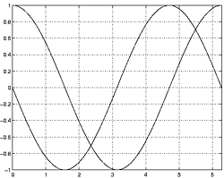
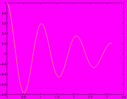
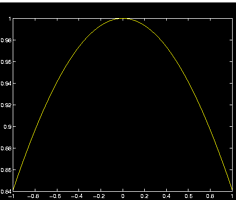
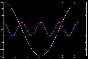
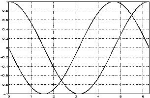
Plot y=sin x + cos 3x over the domain [-p,2p] using steps of p /100:
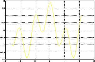
>> x = -pi : pi/100 : 2*pi; y = sin(x)+cos(3*x); plot(x,y),gridNotice there is no need for a dot as we didn't use multiplication, division, or exponentiation of a list.
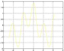
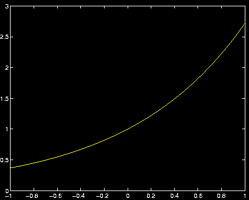
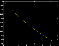
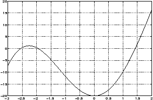
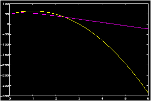
Example: Plot y = e-x/2cos 6x over the domain [0,p]:
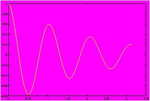
>> x = linspace(0,pi);          % or, x=0:pi/100:pi;
                                % or even (0:100)*(pi/100)
>> y1 = exp(-x/2);              % built in function okay without dot
>> y2 = cos(6*x);               % or, y = (e(-x/2)).*(cos(6*x))
>> y = y1.*y2;                  % need that dot for multiplication
>> plot(x,y),grid
Again note that the dot: ``.'' before the * means that
multiplication of the two arrays y1 and y2 is to be carried
out element-by-element. That is, each element of y is obtained by
multiplying the corresponding elements of y1 and y2.
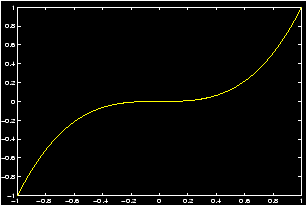
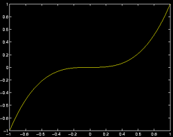
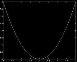
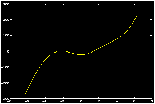
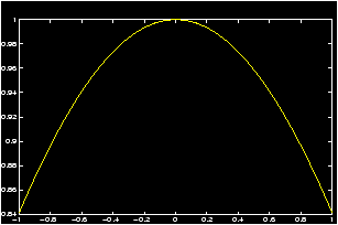
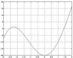
Example: Plot y = x3 over the domain [-1,1]:
>> x = -1 : .05 : 1;            % or use linspace
>> y = x.^3;                    % we need that dot! its a power
>> plot(x,y)
Note again that the dot before the exponentiation means that each element of the x array must be raised to the third power.
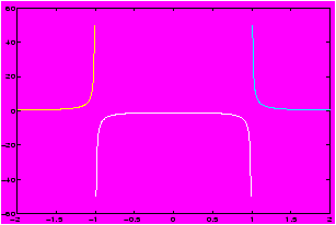
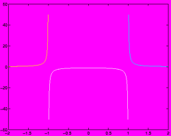
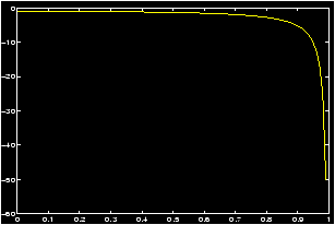
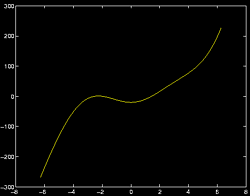
Example: Here is a special example about the syntax of MATLAB. Try this without the parentheses around the 1 before the ./ to see an error message.
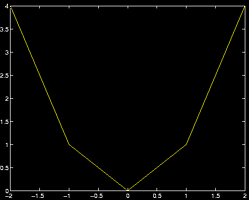
Plot y = 1/(x2-1) over the domain [-2,2]:
>> x = -2 : 0.1 : 2;
>> y = (1)./(x.^2-1);
>> plot(x,y), grid              % notice the discontinuities
You must put the parentheses around the 1 to prevent MATLAB from reading this as
>> y = 1.0/(x.^2 -1)            % dividing by a list needs a dot!!
Try again Homer!
You could avoid having to think this out, if you remember that 1/x = x-1 and use
>> (x.^2 -1).^(-1) % double dots!