Files
der-1.gif
der-2.gif
dt-1.gif
dt-2.gif
dt-20.gif
dt-3.gif
dt-4.gif
fig-1.gif
index.html
lim-1.gif
MatlabPlotting.mp4
MatlabPlottingR2018a.mp4
newtons-method.gif
next_motif.gif
plt-8.gif
plts-1.gif
plts-2.gif
plts-3.gif
plts-4.gif
plts-5.gif
plts-6.gif
plts-7.gif
plts-7a.gif
previous_motif.gif
projectile-motion.mp4
projectile-motionR2018a.mp4
salary.mp4
salaryR2019a.mp4
shrt-1.gif
sin365.mp4
sin365R2018a.mp4
test.gif
tutorial-pieces.html
tutorial.html
tutorial001.gif
tutorial001.html
tutorial002.gif
tutorial002.html
tutorial003.gif
tutorial003.html
tutorial004.gif
tutorial004.html
tutorial005.gif
tutorial005.html
tutorial006.gif
tutorial006.html
tutorial007.gif
tutorial007.html
tutorial008.gif
tutorial008.html
tutorial009.gif
tutorial009.html
tutorial010.gif
tutorial010.html
tutorial011.gif
tutorial011.html
tutorial012.gif
tutorial012.html
tutorial013.gif
tutorial013.html
tutorial014.gif
tutorial014.html
tutorial015.gif
tutorial015.html
tutorial016.gif
tutorial017.gif
tutorial018.gif
tutorial019.gif
tutorial020.gif
tutorial021.gif
tutorial022.gif
zer-1.gif
zer-1a.gif
zer-2.gif
zer-3.gif


8 Limits
Concept: Definition of a limit.
The notion of a limit of a function was originally introduced in order to make the definition of derivative make sense. However, it can also be used to describe the behavior of a function near a given point, as well as to find and describe asymptote s.
One needs to compute limits of the form limx � a f(x) to compute the slope of a tangent line or the derivative of a function, as well as to determine whether a function is continuous.
The definition of a limit of a function, which can be found in any calculus textbook, forms the basis for both a graphical and numerical approach to finding limits.
To summarize it in a means suitable for MATLAB exploration, one has as the value of x gets close to a desired number (often called c), then the value of f(x) gets close to a number L called the limit.
If we want to check out a limit with MATLAB we need to understand this graphically and numerically. Graphically it says if we follow the graph of f(x) towards c from the left or the right, the corresponding y values converge to a limit. Numerically, this says if we look at the sequence of y values corresponding to any sequence of x values which gets close to c then the y values should get very close to a single number -- the limit.
A key result we'll need is that limx � a f(x) = L if and only if both limx � a- f(x) = L and limx � a+ f(x) = L. In other words, we have the following.
The two-sided limit exists if and only if the left- and right-sided limits both exist and are equal.
Thus, to show that the limit is L, essentially we need to show that, as x takes values closer to a (on both sides of a), f(x) takes values closer to L.
-
Example: Finding Limits Graphically
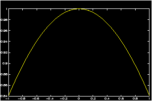
Let us use a graphical approach to determine limx � 0 sin x/x.
Notice this function is not defined at x=0, and ``plugging in'' x=0 gives an indeterminate form of 0/0. Thus the limit takes work to figure out. However, this function is defined for all x except at x=0, which is all that is required to apply the limit definition. The following MATLAB commands will plot the graph of sin x / x near x=0.
  >> x=linspace(-1,1);    % plot for x in the interval [-1, 1]
  >> y=sin(x)./x;         % `dot' makes division point wise
  >> plot(x,y), grid
From the graph you notice as one moves toward 0 from either side on the x-axis, the y values move toward 1. From the graph you can tell what the limit is 1.
-
Example: Finding Limits Numerically
Here is a simple method for finding the same limit numerically.
>> format long                         % gives extra decimal places
>> x=[-.1 -.01 -.001 -.0001 -.00001]   % x approaches 0 from the left
>> y=sin(x)./x; [x;y]'                 % print x,y in a 2-column table
>> x=[.1 .01 .001 .0001 .00001]        % x approaches 0 from the right
>> y=sin(x)./x; [x:y]'
You should get the following results (x on the left, sin (x)/x on the right):ans= -0.10000000000000 0.99833416646828 -0.01000000000000 0.99998333341667 -0.00100000000000 0.99999983333334 -0.00010000000000 0.99999999833333 -0.00001000000000 0.99999999998333 ans= 0.10000000000000 0.99833416646828 0.01000000000000 0.99998333341667 0.00100000000000 0.99999983333334 0.00010000000000 0.99999999833333 0.00001000000000 0.99999999998333Since the values in the right columns both approach 1, we conclude that both right and left limits are 1 and so the limit is 1 as well.
-
Example: limit of slope of the secant line:
See the secant line example to find the definition of the secant line. Essentially we have a function f(x) a point x1 and a point x2. Let x2 = x1 + h. So that h measures the difference between the two values of x. Then as h gets close to 0 x2 and x1 get close to each other. If the limit as h goes to zero exists then the function is said to have a derivative at x1.
In the secant line example we see how to plot the function sin(x) and the secant line between x1 = p/4 and x2 = x1 + h with h = p/8. By changing the value of h we see it is a simple matter to find graphically the limit of the secant lines.
To find the slope numerically we recall the definition of the slope of a linem = (f(x1+h) - f(x1))/(x1 + h - x1) = (f(x1+h) - f(x1))/ hSo in MATLAB we define a sequence of values h converging to 0, and then plug into the formula:>> x_1=pi/4; n = 1:5; h = 10.^(-n); % suppress the output with ; >> m = ( sin(x_1 + h) - sin(x_1)) ./ h; % we need the ./ as h is a % list >> [h;m]' % print out in columnsIf you repeat this using -h in the second and 3rd line you will see that the left and right limits are the same and equal 0.70710 (=2/2).


