---

7   Finding zeroes

In this section we learn several methods for finding zeroes of a function. A brief note on vocabulary is in order.

• If we have an equation, we talk about solutions to the equation: For example the equation sin x = cos x has solutions in [0,2p] given by x = p/4 and x=5p/4.
  
  
• If we have a function f(x) then a zero of f(x) is a value x for which f(x) = 0. To relate to a solution, let f(x) = sin x -cos x. Then the zeroes of f(x) are the solutions to the equation sin x = cos x
  
  
• If we have a polynomial f(x) then the zeroes often get a special name: roots. So, if f(x) = x² + 5x + 6 then the roots of f(x), (x=-3 or x=-2) are the solutions to f(x) = 0.

7.1   Graphically finding zeroes

Here is an example to illustrate how we can find zeroes of a function using the graphing capabilities of MATLAB.


Example: Finding zeroes graphically


Find all solutions of the equation x³ = 20 cos x.
(Notice that this is a non-linear problem, and can't be solved by tricky algebra.)

We have two choices to solve for the solutions graphically. We could plot both the function x³ and the function 20 cos x on the same graph, and then look for points of intersection, or we can take the difference of the two sides, and looks for zeroes of the function f(x) = x³-20cos x. We'll do the latter.

• Let f(x)=x³-20cos x and determine all x values that satisfy the equation f(x)=0. These x values are called the zeros of f or solutions of the equation f(x)=0.
  
  
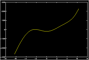
• Create a graph of y=f(x) over a wide domain say from -2p to +2p so that the approximate locations of the roots may be observed.

  >> x=-2*pi:.01:2*pi; y=x.^3-20*cos(x); plot(x,y), grid
  

  ---

  
  
  

  Figure 16: plot over interval [-2p,2p]

  
  

  ---

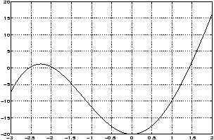
• Examine the resulting graph closely. Since the function 20 cos x is bounded by 20, and |x³| > 20 if x>3, It is evident from the graph that all the solutions are located in the interval [-3,2]. To read their locations more accurately, we create a new plot covering only this interval. Thus changing the range of x accordingly, we enter:

  >> x=linspace(-3,2); 
  >> y=x.^3-20*cos(x);            % redefine y to match new x!
  >> plot(x,y), grid
  

  ---

  
  
  

  Figure 17: plot over the interval [-3,2]

  
  

  ---

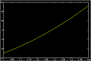
• From this graph we see that nonzero positive solutions are located in the intervals [-2.5,-2], [-2,-1.5] and [1,1.5]. Let us concentrate on the root in [1,1.5]. To read its location more accurately, we create a new plot covering only this interval. Thus changing the range of x we enter:

  >> x=1:.001:1.5; y=x.^3-20*cos(x); plot(x,y), grid
  

  We can now see that the root falls within the interval [1.4,1.5]. We could continue in this fashion and determine the root even more accurately. However, we wish to introduce a new feature of MATLAB which could speed up the determination of the root by zoom ing in and enlarging just the area near the point where the root is located. So, on the command line type:

  >> zoom on
  

  Use the mouse to move the arrow around and point to where the root is located, and click with the left mouse button. The area is enlarged and you can see that the root is slightly greater than 1.42. Repeat this process of pointing to the root and clicking with the left mouse button. After a few repetitions you could approximate the root by x» 1.4255.
  
  How good is this answer? If it is very close to the zero, the value of the function at 1.4255 must be very close to zero. Verify this by entering:

  >> x=1.4255; y=x.^3-20*cos(x)
  

  which results in

   y = 9.7482e-004
  

  It may not appear to be so, but the -004 says this is 0.00097482 which is indeed very close to zero. (You should not expect to get exactly 0 for an answer, as the solution is most likely irrational, and your answer will only be an approximation of the true zero.
  
  When you no longer need the zoom feature, you should turn it off by typing

  >> zoom off
  

7.2   Finding roots of polynomials

Finding zeroes of a polynomial is made easy by the built-in MATLAB command roots .

Example: Finding roots of polynomial
Consider the polynomial f(x)=2x³+6x²-4x-5. To find the roots (or zeroes) of f(x) we graph the function on the interval [-4,3].

>> x=-4:.001:3; y=2*x.^3+6*x.^2-4*x-5;
>> plot(x,y), grid

---

Figure 18: plot of f(x)=2x³+6x²-4x-5

---

There are three real zeros on the intervals [-4,-3], [-1,0] and [1,2]. The values of these roots can be obtained by zooming graphically as was done in this example.

However, for polynomials, MATLAB has a special built-in function roots which can find these roots directly. To use this function one needs first to specify the polynomial in terms of the coefficients of the powers of x.


Example: Example of representing a polynomial with a vector
The polynomial in this example is represented by p=[2 6 -4 -5]. Note that in the array the coefficients are listed in the order of descending powers of x starting with the coefficient of the highest power. (If a particular power of x is not present in the polynomial, then its coefficient is listed as 0. Thus, for example, the polynomial 5x³+2 would be represented by p=[5 0 0 2].) In general, this way of thinking may be of help: Think of the coefficients of the polynomial as then your polynomial is represented by c.

This may be familiar from the ``synthetic division'' technique for finding the value of a polynomial evaluated at c, or dividing f(x) by x-c.

The following sequence of MATLAB commands determine the roots of f(x):

>> p=[2 6 -4 -5];               % place a space or a comma between coefficients
>> r=roots(p)                   % or simply roots([2,6,-4,-5])

which yields the roots:

>> r
  ans  -3.3732   -0.6943  1.0675 % actually a column vector

Concept: Some Theory about Roots of Polynomials
Most math students know that the roots of a 2nd degree polynomial or quadratic polynomial can be found with the quadratic equation . That is if f(x)=ax²+bx+c then the solutions to f(x) = 0 are given by When the discriminant (b² - 4 ac) is negative then there are 2 complex-valued solutions (which are conjugate) and no real solutions (the graph of f(x) does not intersect the x-axis) when the discriminant is 0 there is 1 solution which is a multiple root, and when the discriminant is positive there are two distinct roots. Counting multiplicity then we have the fact that a quadratic polynomial alway has 2 roots.

There are two ways to go from here. First, you may be surprised to know that there are formulas that will give the roots of a third- or a fourth-degree polynomial. However, there is no formula that will work for all fifth- of higher-degree polynomials. (A major feat of mathematics proven in the early 1800's after centuries of effort.)

Secondly, and what is important here, is the Fundamental Theorem of Algebra which states that a polynomial of nth degree will have n roots when we count multiplicities and complex-valued roots.

So when we use the roots command of MATLAB with a nth degree polynomial we have the following: the nth degree polynomial is entered in as a row vector with n+1 elements, and the answer is a column vector with n elements.

You may ask, how does MATLAB find its roots for a polynomial with degree 5 or higher if there is no possible formula. The answer lies in finding good approximations. Newton's method is an old method to find such approximations.

7.3   Newton's method

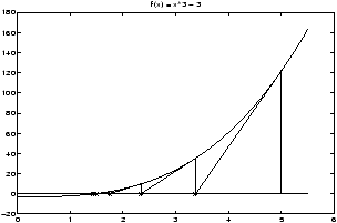
Newton's method is an algorithm to find numeric solutions to the equation f(x) = 0. We have already seen other methods to do this, namely the commands roots for polynomial functions, and the graphical solution .

The general idea idea of Newton's method is easy to understand. Consider the graph of the function f(x) = x³ - 3.

---

Figure 19: Example of convergence of Newton's method

---

By looking at a graph, we see that there is a solution to the equation f(x) = 0 in the interval [0,5]. Call this solution c. Newton's method will help us find a numeric approximation to this value of c. The zig-zagging lines are a graphical representation of the method. Notice how they converge to the desired value of c. These lines were generated as follows. We start at some initial point x₀ (in the picture x₀=5). It should be a reasonable approximation to c. Once we have x₀ we draw a vertical line until we intersect the graph of f(x). Then we follow the tangent line to f until it intersects the x-axis. We use the tangent line because we know it approximates the function quite well near the point (x₀,f(x₀)). This point of intersection is our new guess x₁. This is about 3.3 for the graph. We then repeat, or iterate, this process to find a sequence of points x₂, x₃, and so on. We stop when the new values of x_n don't change too much, or when f(x_n) gets very close to 0.

Given the point x_n, the next point x_n+1 is found by calculating the point at which the tangent line to the graph of f(x) at (x_n,f(x_n)) intersects the x-axis. We know a point, and the slope of this line (it is f'(x_n)) and so this is easy to do. The tangent line in point-slope form has the equation Solving for the x-intercept gives x_n+1:
In MATLAB the subscripts are not used as the equals sign is assignment and not equality. (Consider the difference between x = x+1 and x = x+1.) Thus to apply Newton's method with an initial guess of x₀ = 5 we would simply type

>> format short
>> x = 5                        % our initial guess
>> x = x - (x^3 - 3)./(3*x^2)   % the left x is x_1 the right one x_0
  x = 3.3733                    % x_1
>> x = x - (x^3 - 3)./(3*x^2)   % the left x is x_2 the right one x_1
  x = 2.3368                    % x_2
>> x = x - (x^3 - 3)./(3*x^2)   % the left x is x_3 the right one x_2
  x = 1.7410                    % x_3
.....                           % repeat a few steps
>> x = x - (x^3 - 3)./(3*x^2)   % the left x is x_5 the right one x_6
  x = 1.4423                    % x_6
>> x = x - (x^3 - 3)./(3*x^2)   % the left x is x_7 the right one x_6
  x = 1.4422                    % x_7
>> x = x - (x^3 - 3)./(3*x^2)   % the left x is x_8 the right one x_7
  x = 1.4422                    % x_8

And we see that the solution has converged to 1.4422. Checking that this is a root we evaluate

>> x^3 -3
ans = 0

• Newton's Method can be automated quite easily. An example m-file can be found here: newton.m. To use this, you must first have created m-files for f(x) and f'(x).
• Newton's Method has a few cases where it works quite badly. You may be interested to see why: Here are some examples:
  Example: Too close to a minimum.
  Graphically explore the root that Newton's method finds when
  f(x) = x³ + 2 x² - 30 x -5.
  Compare the graphical output of Newton's method with the following initial points: x₀ = 2,2.20,2,35,2,45. You should see that as the initial guess gets closer to a point on the graph with a 0 derivative, that the method takes much longer to converge.
  Example: Cycling.
  Let f(x) = x³ - 5x. Factor f(x) exactly to find its roots.
  Now use Newton's method with an initial guess of x₀=1. What happens to the subsequent iterations? Can you see what is happening from the graph?
  Now try an initial guess of x₀=2. Does the same problem occur?
  
  
  
  
  Example: Divergence.
  Let f(x) = x^1/3. Clearly x=0 is the only root. By hand (it is easier) compute and simplify f(x)/f'(x). From this compute the sequence of points obtained by Newton's method starting from x₀=1. Is it getting closer to 0?
  
  
• Here is a challenging problem where Newton's method can yield the answer.
  Example: Medical Dosage
  A drug administered to a patient produces a concentration in the blood stream that can be modeled by
  C(t) = Nt e^{- 0.2 t}
  where N is the initial dosage injected in milligrams (mg) and t is the time in hours since the injection. Suppose it is known that the maximum safe concentration of this drug in the blood stream is 2 mg/ml.
  1. When does the maximum concentration occur? Note that the value of N does not affect this answer.
  2. What amount N should be injected so that the maximum concentration is 2 mg/ml? N need not be an integer.
  3. With N from above, suppose that an additional amount of this drug is to be administered to the patient after the concentration falls to 0.25 mg/ml. Determine, to the nearest minute, when this second injection should be given.
  4. Assuming that the concentration from consecutive injections is additive, and assuming that the second injection uses the same amount N of the drug as in the first injection, what will the maximum concentration in the blood stream be after the second injection? Should N be adjusted to ensure that the maximum concentration is still safe?

---